DFT2

1.  Quick recap of DFT

Correlation energy: \(E^C = E^\text{exact}-E^\text{HF}\)

Electron density: \(\rho(r)\)

Functional: \(F[\rho(r)]\), input: function, output: value

Hohenberg-Kohn Theorem:

• \(E[p]\geq E_0, E[p_0]=E_0\)

Kohn-Sham auxiliary system:

\(\hat{H}_\text{aux}=\hat{F}_\text{KS}=-\frac{1}{2}\nabla^2+V_\text{eff}(\vec{r})\)

---

2.  The Kohn-Sham Variational Equations

Slater determinant:

\(H(\vec{x_1},...,\vec{x_N})=\frac{1}{\sqrt{N}}\begin{vmatrix}\theta_1(\vec{x_1}) & ...& \theta_N(\vec{x_1})\\\theta_N(\vec{x_N}) & ...& \theta_N(\vec{x_N})\end{vmatrix}\)

\[\begin{split} &E_\text{KS}[\rho] = \underset{\text{non interacting kinetic}}{T_s[\rho]} + \underset{\text{external potential}}{\int d\vec{F}V_{ne}(\vec{r})\rho(\vec{r})}+ \underset{\text{Classical couomb interaction}}{E_\text{Hartree}[\rho]} + \underset{\text{exchange-correlation}}{E_xc[\rho]}\\ &= -\frac{1}{2} \sum_i^N \int d\mathbf{r}_1\, |\nabla \theta_i(\mathbf{r}_1, \sigma)|^2 - \sum_i^N \int \sum_A^M \frac{Z_A}{|\mathbf{r}_1 - \mathbf{R}_A|} |\theta_i(\mathbf{r}_1)|^2\\ &\quad + \frac{1}{2} \sum_i^N \sum_j^N \int \! \int d\mathbf{r}_1 d\mathbf{r}_2\, |\theta_i(\mathbf{r}_1)|^2 \frac{1}{|\mathbf{r}_1 - \mathbf{r}_2|} |\theta_j(\mathbf{r}_2)|^2 + \underset{\text{unknown}}{E_{\mathrm{xc}}[\rho]} \end{split}\]

Again, the unknown term is \(E_{\mathrm{xc}}[\rho]\). Similarly as what we done in previous Hartree-Fock approximation session, we applied variational principle to make the orbitals \(\theta_i(r)\) fulfill in order to minimize this energy.

Recall that, variational principle \(\theta_i(r)\rightarrow \delta \theta_i(r), \delta \text{ is the variation factor}\)

\[\begin{split} \hat{F}^\text{KS}\theta_i(r_1)=\epsilon \theta_i (r_1)\\ -\frac{1}{2}\nabla_1^2 + V_\text{eff}(r_1) \end{split}\]

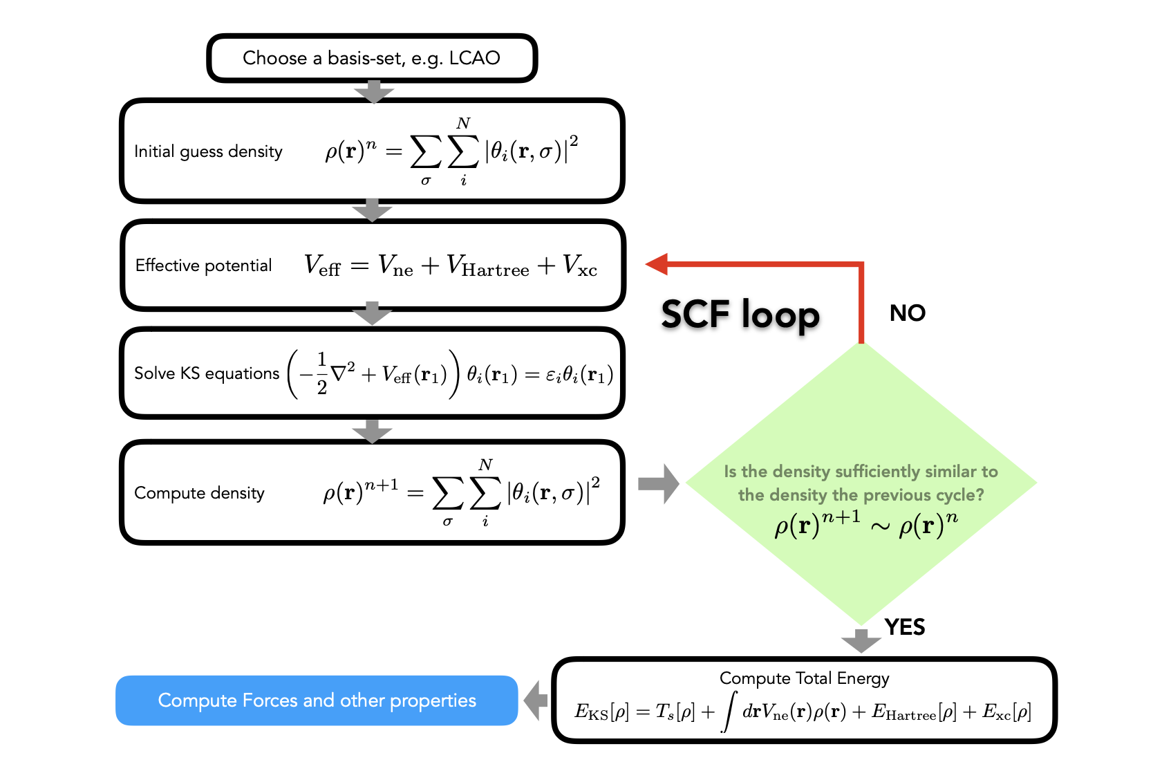
3.  Achieving Self-Consistency of the Kohn-Sham Equations

\[ V_\text{eff} = \underset{\text{constant}}{V_\text{ne}}+\frac{\delta E_H[\rho]}{\delta \rho} +\frac{\delta E_\text{xc}[\rho]}{\delta \rho} \]

4.  Finding the Unknown Exchange-Correlation Functionals

[ \left{ \begin{aligned} &\text{1. Chemist (empirical): get }E_\text{xc}\text{ by comparing to experiments}\ &\text{e.g. heat of formation} \ &\rightarrow\text{ energy does not guarantee a better functional or }\rho \ &\text{2. Physicist: build from scratch (based on feature/constraints)}\ &\rightarrow\text{ limited known features/constraints} \end{aligned} \right. ]

Local Density Approximation (LDA)

Assumption: uniform electron gas (metallic)

\[ E_\text{xc}^\text{LDA}=\int\rho(r)\epsilon_\text{xc}[\rho(r)]dr \]

• where \(\epsilon_\text{xc}\) is the exchange-correlation energy per particle of a uniform electron gas of density \(\rho(r)\).

The quantity \(\epsilon_\text{xc}[\rho(r)]\) exchange and correlation contributions can be spilt as :

\[\begin{split} \epsilon_\text{xc}[\rho(r)] = \underset{\text{exchange}}{\epsilon_\text{x}[\rho(r)]}+ \underset{\text{correlation}}{\epsilon_\text{c}[\rho(r)]}\\ \rightarrow \text{exchange: }\epsilon_x[\rho(r)]=-\frac{3}{4}\sqrt[3]{\frac{3\rho(r)}{\pi}}\\ \rightarrow \text{correlation: no explicit expression:}\\ \text{fit Quantum Monte Carlo} \end{split}\]

Generalized Gradient Approximation (GGA)

\[ E_\text{xc}^\text{GGA}=\int f(\rho, \nabla\rho)dr \]

The gradient itself It’s more like adding a Tylor expansion, the LDA method is the zero order of the series, while the gradient behaves as polynomials, making it more close the to value.

Meta-GGA Rung-3 functional on Jacob’s ladder of DFT. It improves over GGA by using additional semilocal information about the electron density:

\[ E_\text{xc}^\text{meta-GGA} = \int f(\rho,\nabla \rho, \nabla^2 \rho,\tau) \]

• \(\tau = \frac{1}{2}\sum_i|\nabla\psi_i|^2 \rightarrow\) kinetic-energy density

Kinetic energy density physical meanings:

It is large where orbitals oscillate rapidly (e.g. core, bonding), small where density is smooth.

1. bonding type (metallic, ionic, covalent)

2. iso-orbital regions (single-orbital like H atom)

3. weak interactions (vdW regions)