
Pandas#
1. Introduction to pandas Data Structures#
\(\left\{\begin{aligned}&Series\\&DataFrame\end{aligned}\right.\)
1.1. Series#
A Series is a one-dimensional array-like object containing a sequence of values (of similar types to NumPy types) and an associated array of data labels, called its index. The simplest Series is formed from only an array of data:
pd.Series([30, 35, 40], index=['2015 Sales', '2016 Sales', '2017 Sales'], name='Product A')
A Series is, in essence, a single column of a DataFrame. So you can assign row labels to the Series the same way as before, using an index parameter. However, a Series does not have a column name, it only has one overall name :
1.2. DataFrame#
A DataFrame represents a rectangular table of data and contains an ordered collec‐ tion of columns, each of which can be a different value type (numeric, string, boolean, etc.). The DataFrame has both a row and column index; it can be thought of as a dict of Series all sharing the same index. Under the hood, the data is stored as one or more two-dimensional blocks rather than a list, dict, or some other collection of one-dimensional arrays.
A DataFrame is a table. It contains an array of individual entries, each of which has a certain value. Each entry corresponds to a row (or record) and a column.
There are many ways to construct a DataFrame, though one of the most common is from a dict of equal-length lists or NumPy arrays:
data = {'state': ['Ohio', 'Ohio', 'Ohio', 'Nevada', 'Nevada', 'Nevada'],
            'year': [2000, 2001, 2002, 2001, 2002, 2003],
            'pop': [1.5, 1.7, 3.6, 2.4, 2.9, 3.2]}
frame = pd.DataFrame(data)
The list of row labels used in a DataFrame is known as an Index. We can assign values to it by using an index parameter in our constructor:
pd.DataFrame({'Bob': ['I liked it.', 'It was awful.'], 'Sue': ['Pretty good.', 'Bland.']},index=['Product A', 'Product B'])
If you specify a sequence of columns, the DataFrame’s columns will be arranged in that order:
pd.DataFrame(data, columns=['Sue', 'Bob'])
The Series and the DataFrame are intimately related. It’s helpful to think of a DataFrame as actually being just a bunch of Series “glued together”.
2. Indexing, Selecting & Assigning#
2.1. Native accessors#
In Python, we can access the property of an object by accessing it as an attribute. A book object, for example, might have a title property, which we can access by calling book.title. Columns in a pandas DataFrame work in much the same way.
#first way
review.country
#second way
review['country']
2.2. Index in pandas#
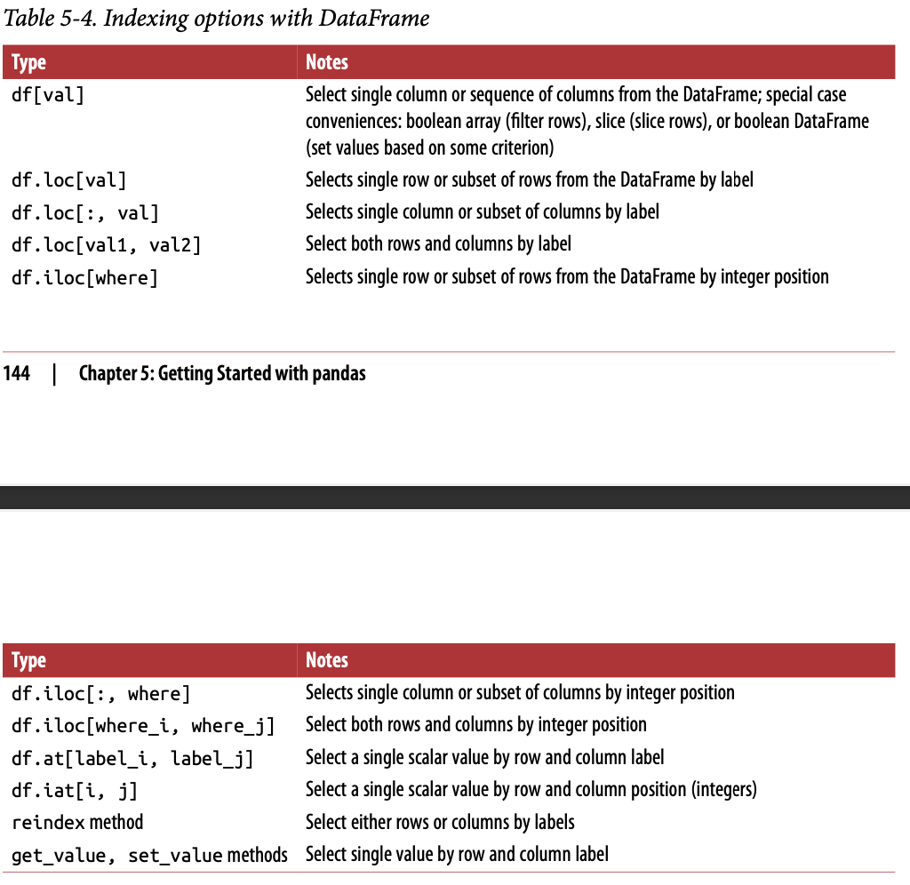
The indexing operator and attribute selection are nice because they work just like they do in the rest of the Python ecosystem. As a novice, this makes them easy to pick up and use. However, pandas has its own accessor operators, loc and iloc. For more advanced operations, these are the ones you’re supposed to be using.
Index-based selection
Selecting data based on its numerical position in the data. iloc follows this paradigm.
Label-based selection
The second paradigm for attribute selection is the one followed by the loc operator: label-based selection. In this paradigm, it’s the data index value, not its position, which matters.
Both loc and iloc are row-first, column-second. This is the opposite of what we do in native Python, which is column-first, row-second.
2.3. Manipulating the index#
Label-based selection derives its power from the labels in the index. Critically, the index we use is not immutable. We can manipulate the index in any way we see fit.
The set_index() method can be used to set the DataFrame index (row labels) using one or more existing columns or arrays (of the correct length). The index can replace the existing index or expand on it.
The reset_index method can reset the index of the DataFrame, and use the default one instead. If the DataFrame has a MultiIndex, this method can remove one or more levels.
2.4. Condition selection#
reviews.country == 'Italy'
reviews.loc[reviews.country == 'Italy']
reviews.loc[(reviews.country == 'Italy') & (reviews.points >= 90)]# & represent and
reviews.loc[(reviews.country == 'Italy') | (reviews.points >= 90)]#|represent or
reviews.loc[reviews.country.isin(['Italy', 'France'])]
reviews.loc[reviews.price.notnull()]
3. Summary Functions and Maps#
3.1. Summary functions#
Pandas provides many simple “summary functions” (not an official name) which restructure the data in some useful way. For example, consider the describe() method:
reviews.points.describe()
count    129971.000000
mean         88.447138
             ...
75%          91.000000
max         100.000000
Name: points, Length: 8, dtype: float64
This method generates a high-level summary of the attributes of the given column. It is type-aware, meaning that its output changes based on the data type of the input. The output above only makes sense for numerical data; for string data here’s what we get:
reviews.taster_name.describe()
count         103727
unique            19
top       Roger Voss
freq           25514
Name: taster_name, dtype: object
If you want to get some particular simple summary statistic about a column in a DataFrame or a Series, there is usually a helpful pandas function that makes it happen.
mean()to see the mean of the points allottedunique()to see a list of unique valuesvalue_counts()to see a list of unique values and how often they occur in the dataset,
3.2. Maps#
A map is a term, borrowed from mathematics, for a function that takes one set of values and “maps” them to another set of values. In data science we often have a need for creating new representations from existing data, or for transforming data from the format it is in now to the format that we want it to be in later. Maps are what handle this work, making them extremely important for getting your work done!
\(\left\{\begin{aligned}&map ()\\&apply ()\end{aligned}\right.\)
map
map() is the first, and slightly simpler one. Used with built-in Python collections like lists, tuples, etc. The function you pass to map() should expect a single value from the Series (a point value, in the above example), and return a transformed version of that value. map() returns a new Series where all the values have been transformed by your function.
review_points_mean = reviews.points.mean()
reviews.points.map(lambda p: p - review_points_mean)
apply
Used with pandas DataFrame or Series.
apply() is the equivalent method if we want to transform a whole DataFrame by calling a custom method on each row.
def remean_points(row):
    row.points = row.points - review_points_mean
    return row

reviews.apply(remean_points, axis='columns')
4. Grouping and Sorting#
4.1. Groupies analysis#
A groupby() operation involves some combination of splitting the object, applying a function, and combining the results. This can be used to group large amounts of data and compute operations on these groups.
reviews.groupby('points').price.min()
Another groupby() method worth mentioning is agg(), which lets you run a bunch of different functions on your DataFrame simultaneously. For example, we can generate a simple statistical summary of the dataset as follows:
reviews.groupby(['country']).price.agg([len, min, max])
You can think of each group we generate as being a slice of our DataFrame containing only data with values that match. This DataFrame is accessible to us directly using the apply() method, and we can then manipulate the data in any way we see fit.
4.2. Multi-index#
All of the examples we’ve seen thus far we’ve been working with DataFrame or Series objects with a single-label index. groupby() is slightly different in the fact that, depending on the operation we run, it will sometimes result in what is called a multi-index.
Multi-indices have several methods for dealing with their tiered structure which are absent for single-level indices. They also require two levels of labels to retrieve a value. Dealing with multi-index output is a common “gotcha” for users new to pandas.
The use cases for a multi-index are detailed alongside instructions on using them in the MultiIndex / Advanced Selection section of the pandas documentation.
countries_reviewed = reviews.groupby(['country','province']).description.agg([len])
countries_reviewed
However, in general the multi-index method you will use most often is the one for converting back to a regular index, the reset_index() method:
countries_reviewed.reset_index()
4.3. Sorting#
we can see that grouping returns data in index order, not in value order. That is to say, when outputting the result of a groupby, the order of the rows is dependent on the values in the index, not in the data.
To get data in the order want it in we can sort it ourselves. The sort_values() method is handy for this.
countries_reviewed=countries_reviewed.reset_index()
countries_reviewed.sort_values(by='len',ascending=False)
# sort by more than one column at a time.
countries_reviewed.sort_values(by=['country', 'len'])
To sort by index values, use the companion method sort_index(). This method has the same arguments and default order.
5. Data Types and Missing Values#
5.1. Dtypes#
The data type for a column in a DataFrame or a Series is known as the dtype.
Data types tell us something about how pandas is storing the data internally. float64 means that it’s using a 64-bit floating point number; int64 means a similarly sized integer instead, and so on.
One peculiarity to keep in mind (and on display very clearly here) is that columns consisting entirely of strings do not get their own type; they are instead given the object type.
It’s possible to convert a column of one type into another wherever such a conversion makes sense by using the astype() function. For example, we may transform the points column from its existing int64 data type into a float64 data type:
In[1]:reviews.price.dtype
Out[1]:dtype('float64')
In[2]reviews.points.astype('float64')
Out[2]0         87.0
			1         87.0
          			...
			129969    90.0
			129970    90.0
			Name: points, Length: 129971, dtype: float64
5.2. Missing data#
Entries missing values are given the value NaN, short for “Not a Number”. For technical reasons these NaN values are always of the float64 dtype.
Pandas provides some methods specific to missing data. To select NaN entries you can use pd.isnull() (or its companion pd.notnull()). This is meant to be used thusly:
reviews[pd.isnull(reviews.country)]
Replacing missing values is a common operation. Pandas provides a really handy method for this problem: fillna(). fillna() provides a few different strategies for mitigating such data. For example, we can simply replace each NaN with an "Unknown":
reviews.region_2.fillna("Unknown")
Alternatively, we may have a non-null value that we would like to replace. For example, suppose that since this dataset was published, reviewer Kerin O’Keefe has changed her Twitter handle from @kerinokeefe to @kerino. One way to reflect this in the dataset is using the replace() method:
reviews.taster_twitter_handle.replace("@kerinokeefe", "@kerino")
6. Renaming and Combining#
rename() lets you rename index or column values by specifying a index or column keyword parameter, respectively. It supports a variety of input formats, but usually a Python dictionary is the most convenient. Here is an example using it to rename some elements of the index.
reviews.rename(columns={'points': 'score'})
reviews.rename(index={0: 'firstEntry', 1: 'secondEntry'})
Both the row index and the column index can have their own name attribute. The complimentary rename_axis() method may be used to change these names. For example:
reviews.rename_axis("wines", axis='rows').rename_axis("fields", axis='columns')
6.1. Combining#
When performing operations on a dataset, we will sometimes need to combine different DataFrames and/or Series in non-trivial ways. Pandas has three core methods for doing this. In order of increasing complexity, these are concat(), join(), and merge(). Most of what merge() can do can also be done more simply with join(), so we will omit it and focus on the first two functions here.
concat() Given a list of elements, this function will smush those elements together along an axis.
join() Combine different DataFrame objects which have an index in common.
left = canadian_youtube.set_index(['title', 'trending_date'])
right = british_youtube.set_index(['title', 'trending_date'])

left.join(right, lsuffix='_CAN', rsuffix='_UK')
The lsuffix and rsuffix parameters are necessary here because the data has the same column names in both British and Canadian datasets. If this wasn’t true (because, say, we’d renamed them beforehand) we wouldn’t need them.