Dimensionality Reduction#
Projection
\(\rightarrow\) training instances are not spread out uniformly across all dimensions. Many features are almost constant, while others are highly correlated
Manifold learning
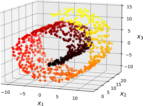
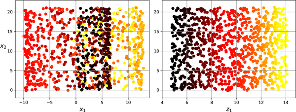
left figure is the projection method, while the right one is the unrolling one. Simply projecting onto a plane (e.g., by dropping \(x_3\)) would squash different layers of the Swiss roll together.
In short, reducing the dimensionality of your training set before training a model will usually speed up training, but it may not always lead to a better or simpler solution; it all depends on the dataset.
1. Principal component analysis(PCA)#
Single value decomposition(SVD)
\(X=U\sum{V^T}\)
\(V \text{ contains the unit vectors that define all the principal components}\)
\(V=\begin{bmatrix} c_1 & 0&0&... \\ 0 & c_2&0&...\\0&0&c_3&... \\0&0&0&... &c_n\end{bmatrix}\)
PCA assumes that the dataset is centered around the origin. As you will see, Scikit-Learn’s PCA classes take care of centering the data for you. If you implement PCA yourself (as in the preceding example), or if you use other libraries, don’t forget to center the data first.
import numpy as np

X = [...]  # create a small 3D dataset
# Center the data first
X_centered = X - X.mean(axis=0)
U, s, Vt = np.linalg.svd(X_centered)
c1 = Vt[0]
c2 = Vt[1]
Projecting down to d dimensions
\(X_{d-proj}=X.W_d\)
\(X_{d-proj} \text{ is the reduced dataset of dimensionality d}\)
\(W_d \text{ is the matrix containing the first d columns of V}\)
W2 = Vt[:2].T
X2D = X_centered @ W2
from sklearn.decomposition import PCA

pca = PCA(n_components=2)
X2D = pca.fit_transform(X)
pca.explained_variance_ratio_
array([0.7578477 , 0.15186921])
Choosing the Right Number of Dimensions
Instead of arbitrarily choosing the number of dimensions to reduce down to, it is simpler to choose the number of dimensions that add up to a sufficiently large portion of the variance—say, 95%
for i
\(Var(X_{d-proj}|X)>95\%\)
\(\sum_{i=0}^{i=n} i\)
PCA for Compression and decompression
This won’t give you back the original data, since the projection lost a bit of information (within the 5% variance that was dropped), but it will likely be close to the original data. The mean squared distance between the original data and the reconstructed data (compressed and then decompressed) is called the reconstruction error.
\(X_{recovered}=X_{d-proj}W_d^T\)
X_recovered =
pca.inverse_transform(X_reduced)
2. Locally linear embedding(LLE)#
Nonlinear dimensionality reduction (NLDR)
It is a manifold learning technique that does not rely on projections, unlike PCA and random projection. In a nutshell, LLE works by first measuring how each training instance linearly relates to its nearest neighbors, and then looking for a low-dimensional representation of the training set where these local relationships are best preserved (more details shortly). This approach makes it particularly good at unrolling twisted manifolds, especially when there is not too much noise.
How its works?
Step1: Linearly modeling local relationships
for each training instance x(i), the algorithm identifies its k-nearest neighbors (in the preceding code k = 10), then tries to reconstruct x(i) as a linear function of these neighbors. More specifically, it tries to find the weights \(w_{i,j}\) such that the squared distance between x(i) and is as small as possible, assuming \(w_{i,j}\) = 0 if x(j) is not one of the k-nearest neighbors of x(i).
\(\sum_{j=1}^m w_{i,j}=1\) for \(i=1,2,....,m\)
Step 2: Reducing dimensionality while preserving relationships
from sklearn.datasets import make_swiss_roll
from sklearn.manifold import LocallyLinearEmbedding

X_swiss, t = make_swiss_roll(n_samples=1000, noise=0.2, random_state=42)
lle = LocallyLinearEmbedding(n_components=2, n_neighbors=10, random_state=42)
X_unrolled = lle.fit_transform(X_swiss)