MolGAN: An implicit generative model for small molecular graphs#
1. Introduction#
Sidestep this issue by utilizing implicit, likelihood-free methods, in particular, a generative adversar- ial network (GAN) that we adapt to work directly on graph representations. We further utilize a reinforcement learning (RL) objective similar to ORGAN (Guimaraes et al., 2017) to encourage the generation of molecules with particular properties.
2. Background#
2.1. Molecular graph#
Undirected graph G with a set of edges \(\xi\) and nodes \(V\) .
Each atoms correspond to a node \(v_i \in V\) that is associated with a T-dimensional one-hot vector \(x_i\)
Represent Atomic bond as an edge \((v_i,v_j)\in \xi\) associate with a bond type \(y\in \) {\(1,...,Y\)}
For molecular graph with N nodes
Node feature matrix \(X=[X_1,...,X_N]^T\in R^{N\times T}\)
Adjacency tensor \(A\in R^{N\times N\times Y}\) where \(A_{ij}\in R^Y\) is a one-hot vector indicating the type of edge between \(i\) and \(j\).
2.2. Generative adversarial networks#
Generative model \(G_\theta\), learns a map from a prior to the data distribution to sample new data-points.
Discriminative model \(D_\phi\), learns to classify whether samples came from the distribution rather than from \(G_\theta\).
Those two models are implemented as neural networks and trained simultaneously with stochastic gradient descent (SGD).
3. Model#
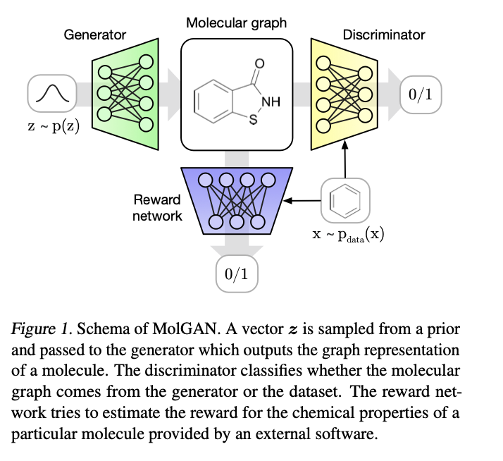
Components: a generator \(G_\theta\) , a discriminator \(D_\phi\) , and a reward network \(\hat{R}_\psi\)
The reward network is used to approximate the reward function of a sample and optimize molecule generation to- wards non-differentiable metrics using reinforcement learning.
3.1. Input of the model#
Generator: \(z \sim p_z(z)\) , A noise vector z sampled from a prior distribution \(p_z(z)\) .
Discriminator: \(x\sim P_{data}(x)\) and \(G_\theta(z)\)
Reward network: Dataset and generated samples are inputs of \(R^\psi\) ,different from discriminator, it assign scores to the molecular graph (e.g., to be easily synthesizable) by RDkit.
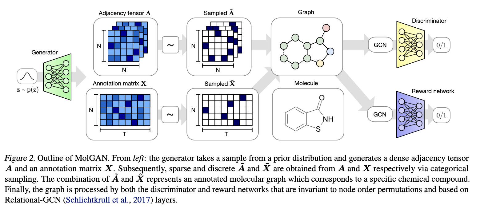
3.2. Generator#
\(z\in R^D\) and \(z \sim \mathcal{N}(0, I) \)
\(z\longrightarrow G_\theta \longrightarrow\left\{\begin{aligned}&X\in R^{N\times T}\\&A^{N\times N\times Y}\end{aligned}\right.\)
Because both X and A have a probabilistic interpretation since each node and edge type is represented with probabilities of categorical distributions over types. To generate a molecule we obtain discrete, sparse objects \(\tilde{X}\) and \(\tilde{A}\) via categorical sampling from X and A, respectively. We overload notation and also represent samples from the dataset with binary \(\tilde{X}\) and \(\tilde{A}\).
As this discretization process is non-differentiable(Two strategies):
i.Use continuous \(X\) and \(A\) directly during the forward pass.
ii. Add Gumbel noise to \(X,A\) before passing to \(D_\phi\) and \(\hat{R}_\psi\).
i.e. \(\tilde{X_{ij}}=X_{ij}+Gum(\mu=0,\beta=1)\),
\(\tilde{A_{ijy}}=A_{ijy}+Gum(\mu=0,\beta=1)\)
iii. Use a straightthrough gradient based on categorical reparameterization with the Gum-softmax.1
i.e. \(\tilde{X_i}=Cat(X_i),\tilde{A_{ij}=Cat(A_{ij})}\)
3.3. Discriminator and reward network#
Both the discriminator \(D_\phi\) and the reward network \(R^\psi\) receive a graph as input, and they output a scalar value each.
A series of graph convolution layers convolve node signals \(\tilde{X}\) using the graph adjacency tensor \(\tilde{A}\). At every layer, feature representations of nodes are convolved/propagated according to:
\(h_i^{(l)}\) is the signal of the node \(i\) at layer \(l\).
\(f_s^{(l)}\) is a linear transformation function that acts as a self connection between layers.
\(f_y^{(l)}\) an edge type-specific affine function for each layer.
\(\mathcal{N}_i\) denotes the set of neighbors for node \(i\).
After several layers of propagation via graph convolutions, we can aggregate node embeddings into a graph level representation vector as:
\(\sigma(x)=1/(1+exp(-x))\text{ is the logistic sigmoid function.}\)
\(i\text{ and }j\) are MLPs with a linear output layer.
\(\odot\) denotes element-wise multiplication.
\(h_{\mathcal{G}}\) is a vector representation of graph \(\mathcal{G}\) and it is further processed by an MLP to produce a graph level scalar output \(\in(-\infin,+\infin)\) for the discriminator and \(\in (0,1)\) for the reward network.
4. Additional information#
Hadamard product(Element-wise multiplication)
For two matrices A and B of the same dimension \(m\times n\), the Hadamard product \(A\odot B\) is a matrix of the same dimension as the operands.
\((A\odot B)_{ij}=(A)_{ij}(B)_{ij}\)