Junction Tree VAE

Junction Tree VAE#

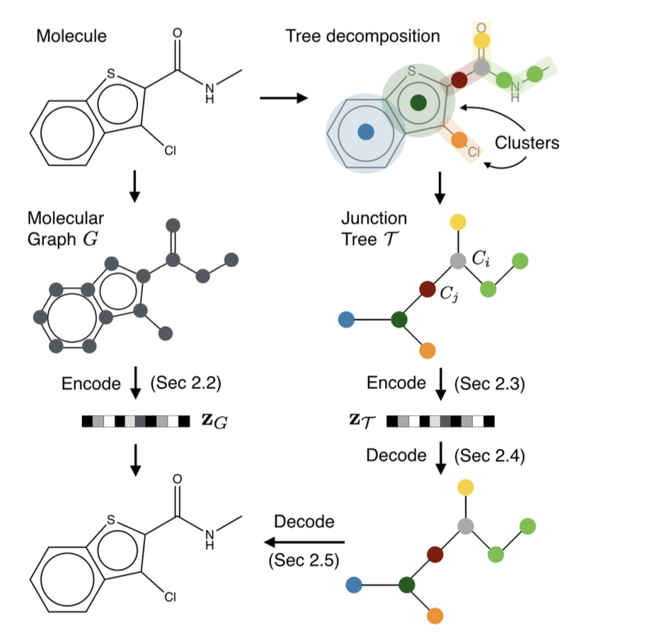
Workflow: Molecular graph $G$ is first decomposed into its junction tree $\mathcal{T}_G$, where each colored node in the tree represents a substructure in the molecule. We then encode both the tree and graph into their latent embeddings $z_\mathcal{T}$ and $z_G$. To decode the molecule, we first reconstruct junction tree from $z_\mathcal{T}$ , and then assemble nodes in the tree back to the original molecule.

So, a molecule is first encoded into 2 parts: $z=[z_\mathcal{T},z_G]$, $\longrightarrow$ Tree encoder $q(z_\mathcal{T},\mathcal{T})$, Graph encoder $q(z_G,G)$

$z_\mathcal{T}$ encodes the tree structure and what the clusters are in the tree without fully capturing how exactly the clusters are mutually connected.
$z_G$ encodes the graph to capture the fine-grained connectivity.

1. Junction Tree#

For a molecular graph $G=(V,E)$

$V$ is the called node of the graph, which is the set of the atoms.
$E$ is called the the edge of the graph, which is set of the bonds of the molecules

A tree decomposition maps a graph $G$ into a junction tree by contracting certain vertices into a single node so that $G$ becomes cycle-free. Formally, given a graph $G$, a junction tree $\mathcal{T}_G = (\mathcal{V},\mathcal{E},\mathcal{X})$ is a connected labeled tree whose node set is $\mathcal{V}= {C_1,···,C_n}$ and edge set is $\mathcal{E}$. Each node or cluster $C_i = (V_i,E_i)$ is an induced subgraph of G, satisfying the following constraints:

2. Graph Encoder#

First encode the latent representation of $G$ by a graph message passing network

For a Graph:

$G=(V,E)$,

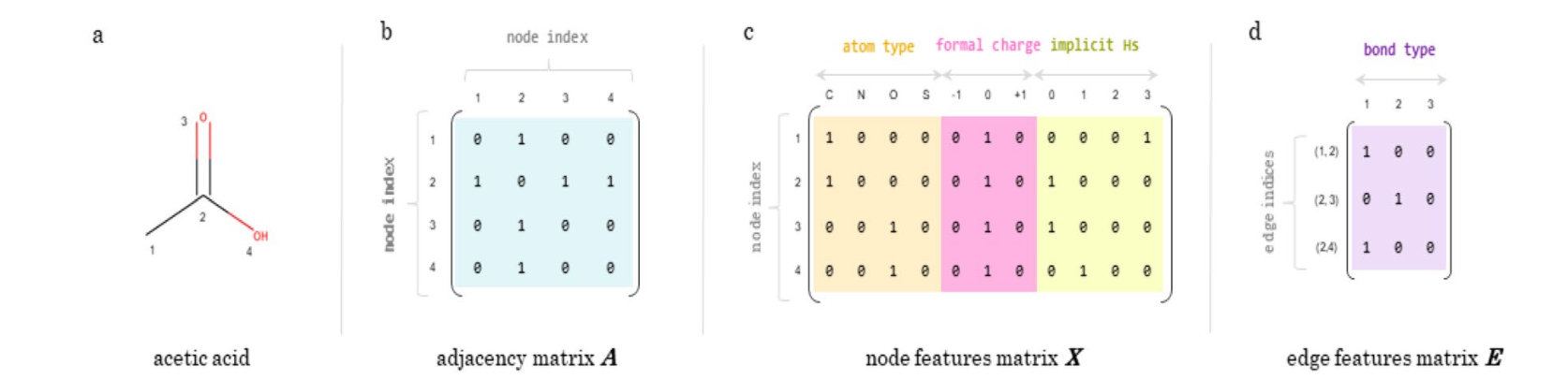
$V$ is the node matrix represent the atoms with features. Each vertex $v$ has a feature vector $\mathbf{x}_v$ indicating the atom type, valence, and other properties.
$E$ is the edge matrix represent the bonds. Each edge $(u,v)\in E$ has a feature vector $\mathbf{x}_{uv}$ indicating the bond type.

Due to the loopy structure of the graph, messages are exchanged in a loopy belief propagation fashion:

\[ \nu_{uv}^{(t)} = \tau \left( \mathbf{W}_1^g \mathbf{x}_u + \mathbf{W}_2^g \mathbf{x}_{uv} + \mathbf{W}_3^g \sum_{w \in \mathcal{N}(u) \setminus v} \nu_{wu}^{(t-1)} \right) \]

$v_{uv}^{(t)}$ is the message computed in $t^{th}$ iteration, initialized with $v_{uv}^{(0)}=0 $

After T steps of iteration, we aggregate those messages as the latent vector of each vertex, which captures its local graphical structure:

\[ \mathbf{h}_u=\tau(\mathbf{U}_1^g\mathbf{x}_u+\sum_{u\in N(u)}\mathbf{U}_2^g\mathbf{\nu}_{uv}^{(T)}) \]

3. Tree Encoder#

This tree encoder plays two roles in our framework. First, it is used to compute $\mathcal{z}_T$, which only requires the bottom-up phase of the network. Second, after a tree $\mathcal{T}$ is decoded from $\mathcal{z}_T$, it is used to compute messages $m_{ij}$ over the entire $\mathcal{T}$, to provide essential contexts of every node during graph decoding.

4. Tree Decoder#

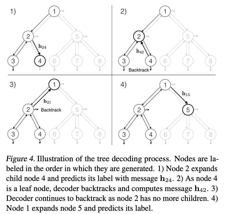
Decode a junction tree $\mathcal{T}$ from its encoding $\mathcal{z}_T$ with a tree structured decoder.

a node receives information from other nodes in the current tree for making those predictions. The information is propagated through message vectors $h_{ij}$ when trees are incrementally constructed.

Assume $\mathcal{E}= \{(i_1,j_1),···,(i_m,j_m)\}$ be the edges traversed in a depth first traversal over $\mathcal{T} = (\mathcal{V},\mathcal{E})$, and $m=2|\mathcal{E}|$ because each edge is traversed in both directions. {% raw %}

\[ \mathbf{h}_{i_t,j_t}=\textbf{GRU}(x_{i_t},\{{\mathbf{h}_{k,i_t}}\}_{(k,i_t)\in \mathcal{E_t},k\ne j_t}) \]

{% endraw %} Topological Prediction When the model visits node it, it makes a binary prediction on whether it still has children to be generated. We compute this probability by combining $\mathcal{z}_T$, node features $x_{i_t}$ and inward messages $h_{k,i_t}$ via a one hidden layer network followed by a sigmoid function to do the binary classification.

\[ p_t=\sigma(\mu^d \cdot \tau (W^d_1 x_{i_t} +W^d_2 \mathcal{z}_T+W^d_3 \sum_{(k,i_t)\in \mathcal{E_t}} h_{k,i_t}) \]

Label Prediction When a child node jis generated from its parent $i$, we predict its node label with

\[ q_j= softmax(U^l\tau(W^l_1\mathcal{z}_T + W^l_2h_{ij})) \]

$q_j$ is a distribution over label vocabulary $\mathcal{X}$.
When $j$ is a root node, its parent $i$ is a virtual node and $h_{ij}= 0$.

Learning

The aim of the decoder is to minimize the likelihood $p(\mathcal{T}|Z_{\mathcal{T}})$

Assume $\hat{p}_t \in\{0,1\}$ and $\hat{q}_j$be the ground truth topological and label values,

the decoder minimizes the following cross entropy loss:

\[ \mathcal{L}_c(\mathcal{T}) = \sum_t\mathcal{L}^d(p_t,\hat{p}_t) + \sum_j\mathcal{L}^l(q_j,\hat{q}_j) \]

4.1. Algorithm 1: Tree Decoding at Sampling Time#

Require: Latent representation $\mathbf{z}_\tau$

Initialize: Tree $\hat{T} \gets \emptyset$
function $SampleTree(i,t)$
Set $\mathcal{X}_i\leftarrow$ all cluster labels that are chemically compatible with node iand its current neighbors.
Set $d_t\leftarrow$ expand with probability $p_t$. $\rightarrow$ equation (4)
if $d_t =$ expand and $\mathcal{X}_i\ne \phi$ then
Create a node $j$ and add it to tree $\hat{\mathcal{T}}$.
Sample the label of node $j$ from $\mathcal{X}_i$ $\rightarrow$ equation (5)
SampleTree$(j,t+ 1)$
end if
end function

5. Graph Decoder#

The final step of our model is to reproduce a molecular graph $\mathcal{G}$ that underlies the predicted junction tree $\mathcal{\hat{T}} = \mathcal{(\hat{V},\hat{E})}$. The underlying degree of freedom pertains to how neighboring clusters $C_i$ and $C_j$ are attached to each other as subgraphs. Our goal here is to assemble the subgraphs (nodes in the tree) together into the correct molecular graph.

Let G(T) be the set of graphs whose junction tree is T. De-coding graph$\hat{G}$ from $\hat{\mathcal{T}} = (\hat{\mathcal{V}},\hat{\mathcal{E}})$ is a structured prediction:

\[ \hat{G} = \arg\max_{G' \in \mathcal{G}(T)} f_a(G') \]

$f_a$ is is a scoring function over candidate graphs.

In other words, each term in the scoring function depends only on how a cluster $C_i$ is attached to its neighboring clusters $C_j$, $j\in N_{\mathcal{\hat{T}}}(i)$ in the tree $\mathcal{\hat{T}}$.

Let $G_iG_i$ be the subgraph resulting from a particular merging of cluster $C_i$ in the tree with its neighbors $C_j$, $j\in N_\mathcal{T}(i)$. We score $Gi$ as a candidate subgraph by first deriving a vector representation $h_{G_i}$ and then using $f_i^a (G_i) = h_{G_i}·z_G$ as the subgraph score. To this end, let $u,v$ specify atoms in the candidate subgraph $G_{i}$ and let $\alpha_v = i $ if $v \in C_i$ and $\alpha_v = j$ if $v \in C_j \setminus C_i.$ The indices αv are used to mark the position of the atoms in the junction tree, and to retrieve messages $m_{i,j}$ summarizing the sub- tree under $i$ along the edge $(i,j)$ obtained by running the tree encoding algorithm. The neural messages pertaining to the atoms and bonds in subgraph $G_{i}$ are obtained and aggregated into $h_{G_i}$ , similarly to the encoding step, but with different (learned) parameters: $$ \mu_{uv}^t=\tau(\mathbf{W}_1^a\mathbf{x}_u+\mathbf{W}2^a\mathbf{x}{uv}+\mathbf{W}3^a\widetilde{\mu}{uv}^{(t-1)})\

\widetilde{\mu}{uv}^{(t-1)}=\left{\begin{aligned} &\sum{w\in N(u)\setminus v}\mu_{wu}^{(t-1)}\qquad &\alpha_u= \alpha_v\ &\mathbf{\hat{m}}{\alpha_u,\alpha_v}+\sum{w\in N(u)\setminus v}\mu_{wu}^{(t-1)}\quad &\alpha_u\ne \alpha_v \end{aligned}\right. $$ The major difference from Eq. (1) is that we augment the model with tree messages $\hat{m}{\alpha_u ,\alpha_v}$ derived by running the tree encoder over the predicted tree $\mathcal{T}$. $\hat{m}{\alpha_u ,\alpha_v}$ provides a tree dependent positional context for bond $(u,v)$

Learning The graph decoder parameters are learned to maximize the log-likelihood of predicting correct subgraphs $G_{i}$ of the ground true graph $G$ at each tree node:

\[ \mathcal{L}_g(G)=\sum_i[f^a(G_i)-\log \sum_{G'\in \mathcal{G_i}}\exp(f^a(G'_i))] \]

$\mathcal{G}_i$ is the set of possible candidate subgraphs at tree node $i$.