Transformer

1.  Introduction

• Eschew recurrence and relying the entirely on the an attention mechanism to draw global dependencies between the input and the output.

• Self-attention (intra-attention), an attention mechanism relating different positions of a single sequence in order to compute a representation of a sequence.

2.  Model Architecture

\(\large\left\{\begin{aligned}Encoder\\\\Decoder\end{aligned}\right.\)

How it works?

​ Encoder: Maps the input sequence of symbol representations (i.e. the text symbols, characters, atoms, thus robust for NLP) \((x_1,x_2,...,x_n)\) to a sequence of continuous representation \((z_1,z_2,...,z_n)\) (this process can be called vectorize process.)

​ **Decoder: **By given the \(z\) ,the decoder can generates an output sequence \((y_1,y_2,...,y_n)\) of symbols one element at a time(this process convert the vector to the symbols type.)

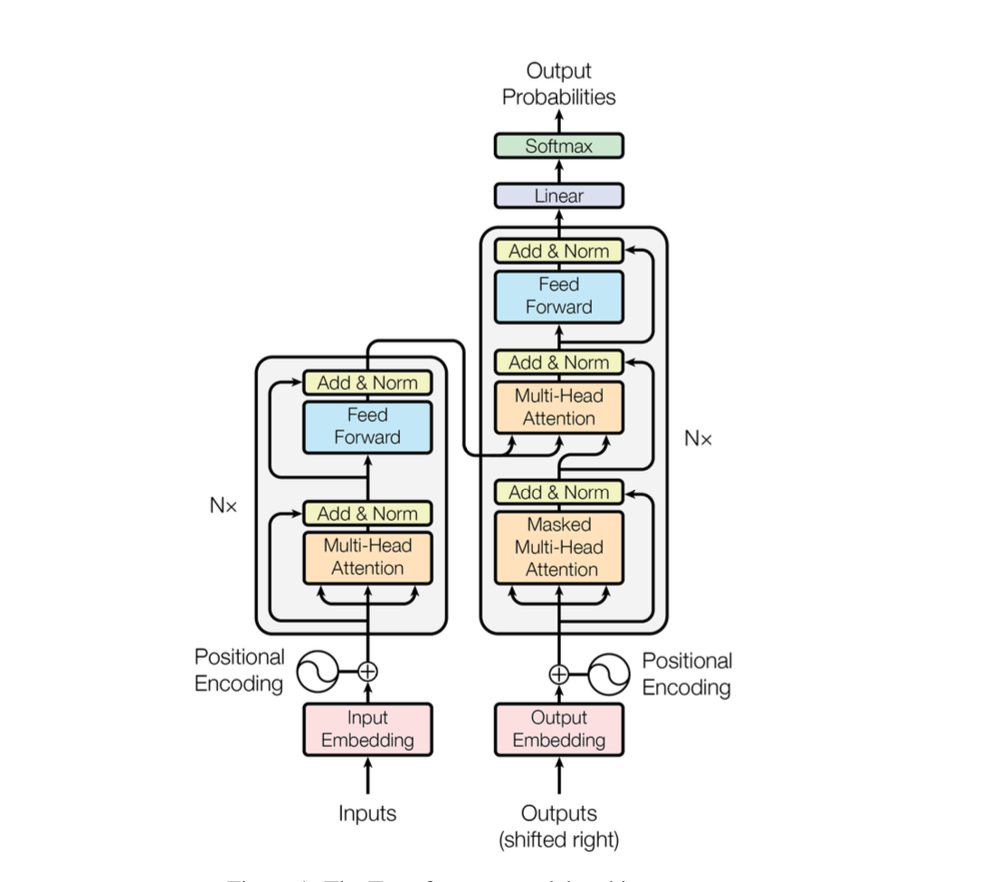
​ Figure 1: The Transformer - model architecture.

2.1.  The structure of Encoder and Decoder

**Encoder: **The encoder is composed of a stack of \(N=6\) identical layers. Each layer has two sub-layers(i.e. Muti-Head attention layer and Feed forward network.) The first is a multi-head self-attention mechanism,and the second is a simple, position wise fully connected feed-forward network. Each of the two sub-layers is employed with a residual connection, followed by layer normalization. Which means the output of each sub-layer should be \(x+ \text{Sublayer}(x)\), where \(\text{Sublayer}(x)\) is the function implemented by the sub-layer itself. The reason why it’s commonly seen that the author introduce high dimension such as \(d_{model} =512\) or 256 and so on in other programs is that higher dimensional outputs of  encoder allows the connections for residual connections, sub-layers in the model, embedding layers and the property distortion procedures.

**Decoder: **The decoder is also composed of a stack of N = 6 identical layers. In addition to the two sub-layers in each encoder layer, the decoder inserts a third sub-layer, which performs multi-head attention over the output of the encoder stack.Similar to the encoder, we employ residual connections around each of the sub-layers, followed by layer normalization. We also modify the self-attention sub-layer in the decoder stack to prevent positions from attending to subsequent positions. This masking, combined with fact that the f, ensures that the predictions for position \(i\) can depend only on the known outputs at positions less than \(i\).

2.2.  Attention

Attention function: Mapping a query and a set of key-value pairs to an output, where the query, keys, values and output are all vectors.

The machine learning-based attention method simulates how human attention works by assigning varying levels of importance to different words in a sentence. It assigns importance to each word by calculating “soft” weights for the word’s numerical representation, known as its embedding, within a specific section of the sentence called the context window to determine its importance. The calculation of these weights can occur simultaneously in models called transformers, or one by one in models known as recurrent neural networks. Attention (machine learning)

• Soft weights: Can adapt and change with each use of the model.

• Hard weights: They are predetermined and fixed during training

Softmax activation function

The softmax function takes as input a vector z of K real numbers, and normalizes it into a probability distribution consisting of K probabilities proportional to the exponentials of the input numbers. That is, prior to applying softmax, some vector components could be negative, or greater than one; and might not sum to 1; but after applying softmax, each component will be in the interval, and the components will add up to 1, so that they can be interpreted as probabilities. Furthermore, the larger input components will correspond to larger probabilities.

Formally, the standard(unit) softmax function \(\sigma:\mathbb{R}^K\rightarrow(0,1)^K,\text{where K}\ge1\), takes a vector \(z=(z_1,...,z_K)\in\mathbb{R}^K\) and computes each components of vector \(\sigma(z)\in(0,1)^K\) within:

\[ \hat{\mathcal{p}_i}=\sigma(z)_i=\frac{e^{z_i}}{\sum^K_{j=1}e^{z_j}} \]

• \(\sigma(z)_i\) is the estimated probability that the instance i belongs to class z, given the scores of each class for that instance.

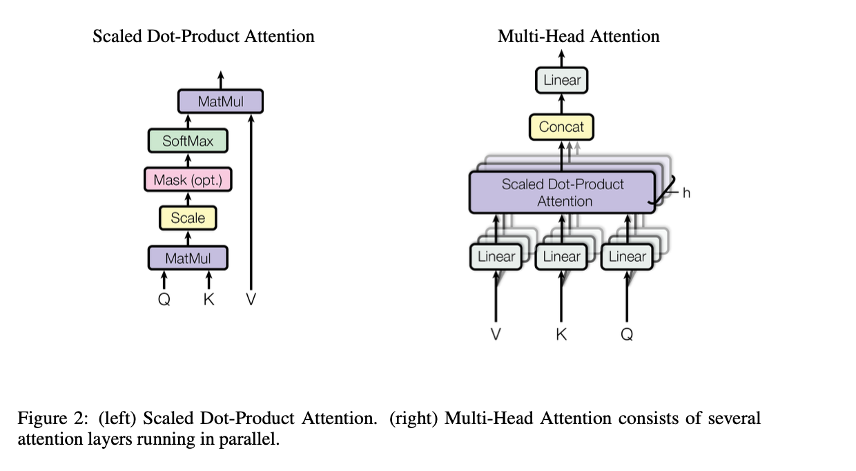
Scaled Dot-Product Attention

The input consists of queries and keys of dimension \(d_k\), and values of dimension \(d_v\). Computing the dot products of the query with all keys, divide each by \(\sqrt{d_k}\) (This process helps to keep the variance of the dot products at a manageable level, ensuring that the softmax function produces a more balanced distribution of attention weights. The magnitude is normalized.) and apply softmax function to obtain the weights on the values.

\[ \text{Attention}(Q,K,V)=\text{softmax}(\frac{QK^T}{\sqrt{d_k}})V \]

[!NOTE]

To illustrate why the dot products get large

Assume: \(q\in Q, Q(\mu,\sigma^2),\mu=,\sigma^2=1\)

​ \(k\in K, K(\mu,\sigma^2),\mu=,\sigma^2=1\)

​ Q is independent with K

​ \(W=q.k=\sum_{i=1}^{d_k} q_ik_i\)

​ \(W(\mu,\sigma^2),\mu=0,\sigma^2=d_k\)

Multi-Head Attention

Multi-head attention allows the model to jointly attend to information from different representation subspaces at different positions.

\[\begin{split} \text{Multihead}(Q,K,V)=\text{concat}(head_1,...,head_h)W^O\\ head_i=\text{Attention}(QW_i^Q,KW_i^K,VM_i^V) \end{split}\]

Projections are parameter matrices:

\(W_i^Q\in \mathbb{R}^{d_{model}\times d_Q},W_i^K\in \mathbb{R}^{d_{model}\times d_K},W_i^V\in \mathbb{R}^{d_{model}\times d_V}\text{ and }W^O\in \mathbb{R}^{{hd_v}\times d_{model}}\)

• h is the parallel attention layer, or heads, it aims to reduce the dimension of each head, if dimension is 512, h is 8, then each layer just needs to deal with 64 dimensions.

Position-wise Feed -Forward Networks

In addition to attention sub-layers, each of the layers in encoder and decoder contains a fully connected feed-forward network, which is applied to each position separately and identically. This consists of two linear transformations with a ReLU activation in between.

\[ FFN(x)=max(0,xW_1+b_1)W_2+b_2 \]

While the linear transformations are the same across different positions, they use different parameters from layer to layer.

ReLU (rectified linear unit)

\[\begin{split} f(x)=x^+=max(0,x)=\frac{x+|x|}{2}=\left\{\begin{aligned}&x,\text{ if } x>0\\&0,\text{ Otherwise}\end{aligned}\right. \end{split}\]

Positional Encoding

Since the model contains no recurrence and no convolution, in order for the model to make use of the order of the sequence, we must inject some information about the relative or absolute position of the tokens in the sequence. To this end, we add “positional encodings” to the input embeddings at the bottoms of the encoder and decoder stacks. The positional encodings have the same dimension \(d_{model}\) as the embeddings, so that the two can be summed. There are many choices of positional encodings, learned and fixed.

\[\begin{split} &PE(pos,2i)=sin(pos/10000^{2i/d_{model}})\\ &PE(pos,2i+1)=cos(pos/10000^{2i/d_{model}}) \end{split}\]

Where:

• pos is the position

• i is the dimension

The wavelengths form a geometric progression from 2π to 10000 · 2π. We chose this function because we hypothesized it would allow the model to easily learn to attend by relative positions, since for any fixed offset \(k, PE_{pos}+k\) can be represented as a linear function of \(PE_{pos}\).