Introduction#
Feature: Each piece of information included in the representation
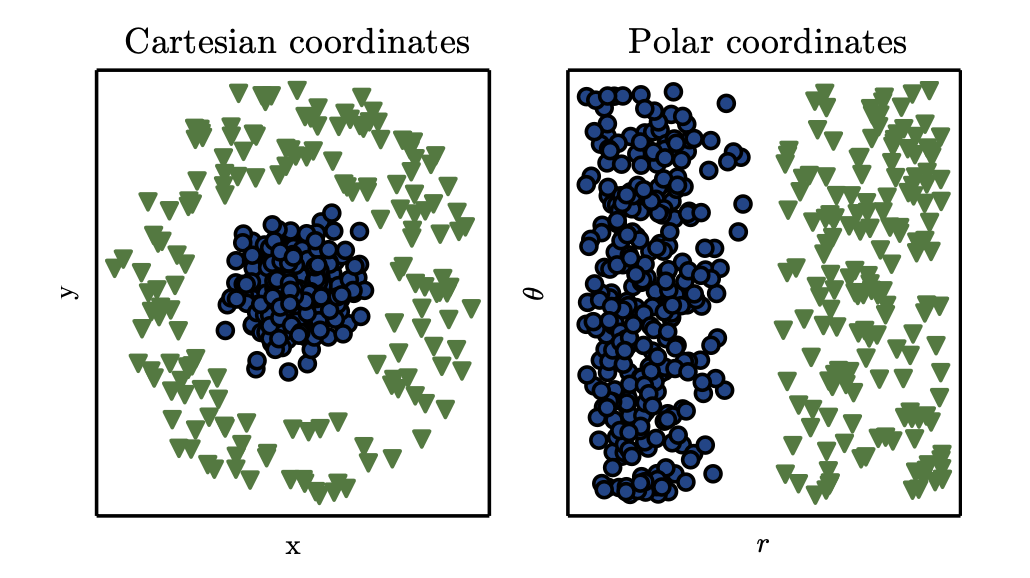
Example of different representations: suppose we want to separate two categories of data by drawing a line between them in a scatterplot. In the plot on the left, we represent some data using Cartesian coordinates, and the task is impossible. In the plot on the right, we represent the data with polar coordinates and the task becomes simple to solve with a vertical line. (Figure produced in collaboration with David Warde-Farley.)
Representation learning: use machine learning to discover not only the mapping from representation to output but also the representation itself
When designing features or algorithms for learning features, our goal is usually to separate the factors of variation
“factors” simply to refer to separate sources of influence
3. Probability Theory#
1. 3.1. Random Variables#
A random variable is a variable that can take on different values randomly.
2. 3.2. Probability Distributions#
A probability distribution is a description of how likely a random variable or set of random variables is to take on each of its possible states. The way we describe probability distributions depends on whether the variables are discrete or continuous.
2.1. 3.2.1. Discrete Variables and Probability Mass Functions#
probability mass function(PMF): A probability distribution over discrete variables
The probability that x = x is denoted as P(x):
\(P=1 \rightarrow \text{x} = x\text{ is certain}\\ P=0 \rightarrow \text{x} = x\text{ is impossible}\)
Denoted as \(P(\text{x} = x)\) or \(x\sim P(x)\)
Joint probability distribution:
Probability mass functions can act on many variables at the same time.
\(P(\text{x} = x,\text{y}= y)\longrightarrow \text{x} = x \quad and \quad \text{y}= y\) simultaneously
uniform distribution:
make each of its states equally likely
\(P(x=x_i)=\frac{1}{k}\) , \(k\) is the constant
To be a PMF on a random variable x, a function P must satisfy the following properties:
The domain of \(P\) must be the set of all possible states of x.
\(\forall x\in\text{x},0\le P(x)\le1.\) An impossible event has probability 0, and no state can be less probable than that. Likewise, an event that is guaranteed to happen has probability 1, and no state can have a greater chance of occurring.
\(\sum_{x\in\text{x}}P(x)=1\). We refer to this property as being normalized. Without this property, we could obtain probabilities greater than one by computing the probability of one of many events occurring.
2.2. 3.2.2. Continuous Variables and Probability Density Functions#
When working with continuous random variables, we describe probability distributions using a probability density function (PDF) rather than a probability mass function.
To be a probability density function, a function p must satisfy the
following properties:
The domain of \(p\) must be the set of all possible states of x.
\(\forall x \in \text{x}, p(x)\ge0.\) Note that we do not require \(p(x)\le 1\)
\(\int p(x)dx=1\)
A probability density function p(x) does not give the probability of a specific state directly; instead the probability of landing inside an infinitesimal region with volume δx is given by \(p(x)\delta x\).
3. 3.3. Marginal Probability#
Sometimes we know the probability distribution over a set of variables and we want to know the probability distribution over just a subset of them. The probability distribution over the subset is known as the marginal probability distribution.
e.g. Suppose we have discrete random variables x and y, and we know \(P(x,y)\).
For discrete random variables:
\(\forall x \in \text{x}, P(\text{x}=x)=\sum_yP(x=\text{x},y=\text{y})\)
For continuous variables:
\(p(x)=\int p(x,y)dy\)
4. 3.4. Conditional Probability#
In many cases, we are interested in the probability of some event, given that some other event has happened. This is called a conditional probability.
The conditional probability is only defined when \(P(\text{x} = x) >0\).
4.1. 3.4.1. The Chain Rule of Conditional Probabilities#
Any joint probability distribution over many random variables may be decomposed into conditional distributions over only one variable:
4.2. 3.4.2. Independence and Conditional Independence#
Two random variables x and y are independent if their probability distribution can be expressed as a product of two factors, one involving only x and one involving only y:
\(\text{x}\perp \text{y}\) means x and y are independent.
\(\text{x}\perp\text{y}\mid\text{z}\) means that x and y are conditionally independent given z.
5. 3.5. Expectation, Variance and Covariance#
Expectation (Expectation value)
Expectation is the average, or mean value, that the function f(x) with respect to a probability distribution P(x) takes on when x is drawn from P.
For discrete variables:
For continuous variables:
[!NOTE]
Expectations are linear, for example: \(\mathbb{E}_x[\alpha f(x)+\beta g(x)]=\alpha\mathbb{E}_x[f(x)]+\beta \mathbb{E}_x[g(x)]\)
Variance
The variance gives a measure of how much the values of a function of a random variable x vary as we sample different values of x from its probability distribution:
When the variance is low, the values of f(x) cluster near their expected value. The square root of the variance is known as the standard deviation.
Covariance
The covariance gives some sense of how much two values are linearly related to each other, as well as the scale of these variables:
\(\text{Cov}(x,y)>0\), positive proportion relation
\(\text{Cov}(x,y)<0\), negative proportion relation
Correlation
Normalize the contribution of each variable in order to measure only how much the variables are related, rather than also being affected by the scale of the separate variables.
6. 3.6. Common Probability Distributions#
6.1. 3.6.1.#
The **Bernoulli distribution **is a distribution over a single binary random variable. It is controlled by a single parameter φ∈[0,1], which gives the probability of the random variable being equal to 1. It has the following properties:
6.2. 3.6.2. Multinoulli Distribution#
The multinoulli, or categorical, distribution is a distribution over a single discrete variable with k different states, where k is finite. The multinoulli distribution is parametrized by a vector \(p\in[0,1]^{k−1}\), where pi gives the probability of the \(i\)-th state. The final, \(k\)-th state’s probability is given by \(1-1\top p\le1\). Note that we must constrain \(1\top p\le1\). Multinoulli distributions are often used to refer to distributions over categories of objects, so we do not usually assume that state 1 has numerical value 1, and so on. For this reason, we do not usually need to compute the expectation or variance of multinoulli-distributed random variables.
6.3. 3.6.3. Gaussian Distribution#
The most commonly used distribution over real numbers is the normal distribution, also known as the Gaussian distribution:
\(\mu\) is the mean of the distribution:\(\mathbb{E}[x]=\mu\)
\(\sigma\) standard deviation of the distribution, and \(\sigma^2\) is the variance
Multivariate normal distribution
When the normal distribution generalizes to \(\mathbb{R}^n\), it may be parametrized with a positive
definite symmetric matrix \(\Sigma\)
parameter \(\mu\) still gives the mean of the distribution
parameter \(\Sigma\) gives the covariance matrix of the distribution.
6.4. 3.6.4. Exponential and Laplace Distributions#
Exponential distribution
In the context of deep learning, we often want to have a probability distribution with a sharp point at x = 0. To accomplish this, we can use the exponential distribution:
The exponential distribution uses the indicator function \(\mathbf{1}_{x\ge0}\) to assign probability zero to all negative values of x.
Laplace distribution
A closely related probability distribution that allows us to place a sharp peak of probability mass at an arbitrary point \(\mu\) is the Laplace distribution
6.5. 3.6.5. The Dirac Distribution and Empirical Distribution#
In some cases, we wish to specify that all the mass in a probability distribution clusters around a single point. This can be accomplished by defining a PDF using the Dirac delta function, \(\delta(x)\):
A common use of the Dirac delta distribution is as a component of an empirical distribution,
which puts probability mass \(\frac{1}{m}\) on each of the \(m\) points \(x^{(1)}\ldots x^{(m)}\), forming a given data set or collection of samples. The Dirac delta distribution is only necessary to define the empirical distribution over continuous variables. For discrete variables, the situation is simpler: an empirical distribution can be conceptualized as a multinoulli distribution, with a probability associated with each possible input value that is simply equal to the empirical frequency of that value in the training set.
6.6. 3.6.6. Mixtures of Distributions#
One common way of combining distributions is to construct a mixture distribution. A mixture distribution is made up of several component distributions. On each trial, the choice of which component distribution should generate the sample is determined by sampling a component identity from a multinoulli distribution:
7. 3.7. Useful Properties of Common Functions#
Certain functions arise often while working with probability distributions, especially the probability distributions used in deep learning models.
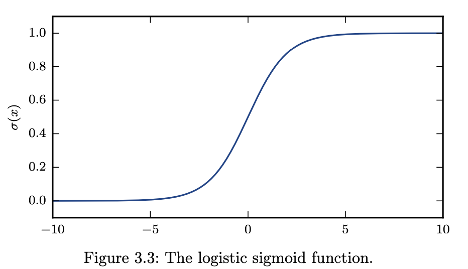
7.1. 3.7.1. Logistic sigmoid#
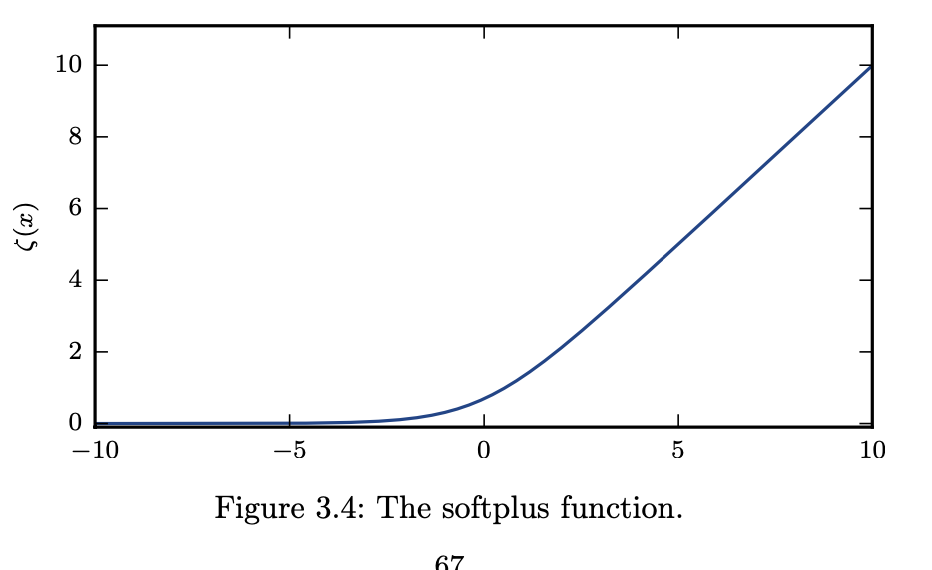
7.2. 3.7.2. Softplus function#
The softplus function can be useful for producing the β or σ parameter of a normal distribution because its range is (0,∞).
8. 3.8. Bayes’ Rule#
To find \(P(x|y)\) when we already know the \(p(y|x)\) and \(p(x)\)
Even \(P(y)\) appears in the formula, we can substituted it: \(P(y)=\sum_xP(y|x)P(x)\)
9. 3.9. Structured Probabilistic Models#
Machine learning algorithms often involve probability distributions over a very large number of random variables. Often, these probability distributions involve direct interactions between relatively few variables. Using a single function to describe the entire joint probability distribution can be very inefficient (both computationally and statistically).
Using a single function to represent a probability distribution. False
Split a probability distribution into many factors that we multiply together True
Suppose we have three random variables: a, b and c. Suppose that a influences the value of b, and b influences the value of c, but that a and c are independent given b.
[!NOTE]
These factorizations can greatly reduce the number of parameters needed to describe the distribution. Each factor uses a number of parameters that is exponential in the number of variables in the factor.
Here, we use the word “graph” in the sense of graph theory: a set of vertices that may be connected to each other with edges. When we represent the factorization of a probability distribution with a graph, we call it a structured probabilistic model, or graphical model.
Directed models use graphs with directed edges, and they represent factorizations into conditional probability distributions. Specifically, a directed model contains one factor for every random variable \(x_i\) in the distribution, and that factor consists of the conditional distribution over \(x_i\) given the parents of \(x_i\), denoted \(Pa_\mathcal{G}(x_i)\):
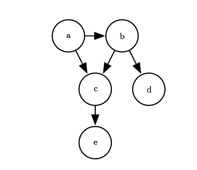
e.g. \(p(a,b,c,d,e) = p(a)p(b\mid a)p(c\mid a,b)p(d\mid b)p(e\mid c). \)
Undirected models use graphs with undirected edges, and they represent factorizations into a set of functions (not not probability distributions of any kind). Any set of nodes that are all connected to each other in \(\mathcal{G}\) is called a clique. Each clique \(C^{(i)}\) in an undirected model is associated with a factor \(\phi^{(i)}(\mathcal{C}^{(i)})\).
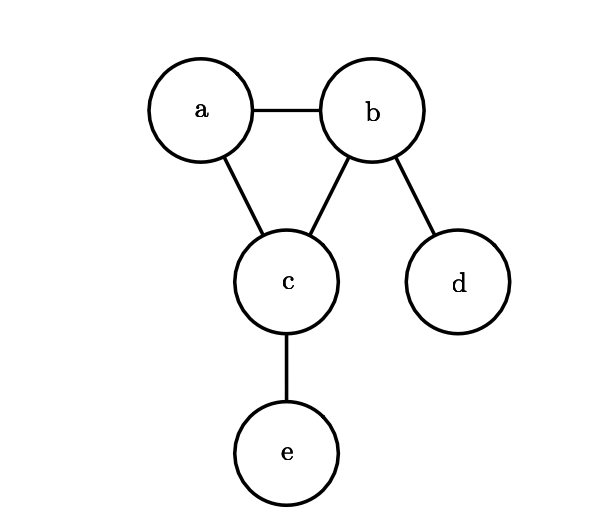
e.g. \(p(a,b,c,d,e)=\frac{1}{Z}\phi^{(1)}(a,b,c)\phi^{(2)}p(b,d)\phi^{(3)}p(c,e)\)
4. Information Theory#
Information theory is a branch of applied mathematics that revolves around quantifying how much information is present in a signal. In the context of machine learning, we can also apply information theory to continuous variables where some of these message length interpretations do not apply. Information theory tells how to design optimal codes and calculate the expected length of messages sampled from specific probability distributions using various encoding schemes.
The basic intuition behind information theory is that learning that an unlikely event has occurred is more informative than learning that a likely event has occurred.
We would like to quantify information in a way that formalizes this intuition.
Likely events should have low information content, and in the extreme case, events that are guaranteed to happen should have no information content whatsoever.
Less likely events should have higher information content.
Independent events should have additive information. For example, finding out that a tossed coin has come up as heads twice should convey twice as much information as finding out that a tossed coin has come up as heads once.
Self-information
\(I(x)=-\log{P(x)}\)
But one problem comes out, if x is continuous instead of discrete, we apply this self information theory, some properties will get lost. Eg. An event with unit density(p(x)=1), still have 0 information, despite this event is not guaranteed to occur.
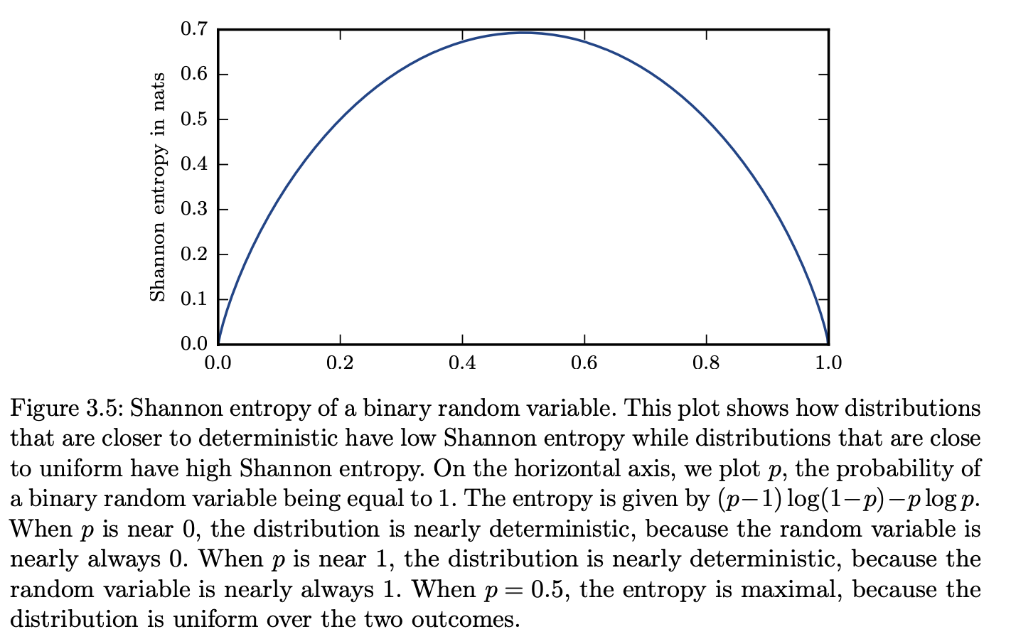
Shannon entropy
Self-information deals only with a single outcome. We can quantify the amount of uncertainty in an entire probability distribution using the Shannon entropy, also denoted \(H(P)\).
Kullback-Leibler (KL) divergence:
The KL divergence has many useful properties, most notably being non-negative. The KL divergence is 0 if and only if P and Q are the same distribution in the case of discrete variables, or equal “almost everywhere” in the case of continuous variables.
5. Numerical Computation#
1. 5.1. Overflow and Underflow#
In ML, we need to represent infinitely many real numbers with a finite number of bit patterns, we incur some approximation error when we represent the number in the computer, rounding error will be accumulated for many operations like the algorithms.
Underflow: Underflow occurs when numbers near zero are rounded to zero.
Overflow: Overflow occurs when numbers with large magnitude are approximated as \(-\infty\) or \(\infty\)
To stabilize the underflow or the overflow, normalization should be applied to reduce the magnitude.
Softmax function
2. 5.2. Poor Conditioning#
Conditioning refers to how rapidly a function changes with respect to small changes in its inputs. Functions that change rapidly when their inputs are perturbed slightly can be problematic for scientific computation because rounding errors in the inputs can result in large changes in the output.
Suppose \(Ax=b\), for perturbation introduced (rounding errors in inputs), \(b=b_0+\Delta b\), when \(A \in \mathbb{R}^{n\times n}\) has an eigenvalue decomposition
\(\Delta x=A^{-1}\Delta b,\rightarrow ||\Delta x||\leq||A^{-1}||\cdot||\Delta b||\\ ||b||\leq ||A||\cdot||x||\\ \frac{||\Delta x||}{||x||}\leq ||A||\cdot ||A^{-1}||\frac{||\Delta b||}{||b||}\)
Condition number
This is the ratio of the magnitude of the largest and smallest eigenvalue. When this number is large, matrix inversion is particularly sensitive to error in the input.
3. 5.3. Gradient-Based Optimization#
Optimization refers minimize or maximize a function \(f(x)\) by adjusting \(x\). (Minimization is standard; maximization is achieved by minimizing \(−f(x)\))
Function to optimize: objective function (also called cost, loss, or error function).
\(x^∗=\) arg min \(f(x)\)
Suppose we have a function y= f(x), where both x and y are real numbers.
The derivative indicates how a small change in \(x\) affects y:
\(f(x+\epsilon)\approx f(x)+\epsilon f^′(x)\)
This property is useful for minimizing f(x) as it shows how to adjust x to reduce y.
Gradient Descent:
A technique to minimize \(f(x)\) by moving \(x\) in small steps opposite to the sign of the derivative.
\(f(x-\epsilon \text{sign}(f'(x)))< f(x)\text{ for small }\epsilon\)
For functions with multiple inputs, we must make use of the concept of partial derivatives. The partial derivative \(\frac{\partial }{\partial x_i}f(x)\) measures how \(f\) changes as only the variable \(x_i\) increases at point \(x\). The gradient generalizes the notion of derivative to the case where the derivative is with respect to a vector: the gradient of \(f\) is the vector containing all the partial derivatives, denoted \(\nabla xf(x)\). Element \(i\) of the gradient is the partial derivative of \(f\) with respect to \(x_i\). In multiple dimensions, critical points are points where every element of the gradient is equal to zero.
The directional derivative in direction \(u\) (a unit vector) is the slope of the function \(f\) in direction \(u\).
gradient descent/method of steepest descent
Where:
\(\epsilon\) is the learning rate, a positive scalar determining the size of the step.
We can choose ϵin several different ways.
set \(\epsilon\) to a small constant, Sometimes, we can solve for the step size that makes the directional derivative vanish.
Evaluate \(f(x-\epsilon \nabla_x f(x))\) for several values of \(\epsilon\) and choose the one that results in the smallest objective function value. Which is called line search.