DFT in solids#
1. Recap of DFT#
1. Kohn-sham equation (Auxiliary method)
3. \(\mathbf{E_{xc}[\rho]}\)
LDA: uniform electron gas \(E_{xc}^{LDA}-\int\rho(\vec{r})\epsilon_{xc}[\rho(\vec{r})]d\vec{r}\)
\(\epsilon_{xc} = \underset{\text{exchange}}{\underbrace{\epsilon_x}} + \underset{\text{correlation}}{\underbrace{\epsilon_c}}\)
e.g. VWN, PZ, PWQ, SPZ
Effective but over-binding
GGA: add \(\nabla \rho(\vec{r})\) (Non-homogeneity)
\(E_\text{xc}^\text{GGA} = \int f(\rho,\nabla \rho)d\vec{r}= E_\text{x}^\text{GGA}(\rho) +E_\text{c}^\text{GGA}(\rho)\)
e.g. PBE, BLYP, …
Very good property results, mostly used for geometries, energies.
self interaction problem
In HF, \(E_x^{HF}+E_H = 0\) , when \(i=j\) (Cancelled)
In DFT, not fully cancelled out.
Hybrid functional:
Mix DFT with HF
e.g. B3LYP: adjustable parameters
PBEO: \(25\% E_x^{HF} + 75\% E_x^{PBE} + E_c^{PBE}\)
HSE06: adjustable parameters, solid
4. Jacob ladder:
\(\text{LDA}\rightarrow \text{GGA}\rightarrow \text{meta-GGA} \rightarrow \text{hybrid functional}\rightarrow \text{exact solution}\)
2. Periodic structures#
[!NOTE]
The Bravais Lattice: The positions and types of atoms in the primitive cell form the basis. The set of translations, which generate the entire periodic crystal by repeating the basis, is a lattice of points in space called the Bravais Lattice.
Primitive Cell:
Smallest unit cell
Fill whole space through translation
It has a single lattice point
Wigner-Seitz unit cell (unique primitive cell):
Translation:
Primitive lattice vector: \(\vec{a_1} &= (0,\frac{1}{2},\frac{1}{2})\\ \vec{a_2}&=(\frac{1}{2},0,\frac{1}{2})\\\vec{a_3}&=(\frac{1}{2},\frac{1}{2},0)\) Conventional lattice vector: \(\vec{a_1} &= (1,0,0)\\ \vec{a_2}&=(0,1,0)\\\vec{a_3}&=(0,0,1)\)
Volume:
\(d=1,& |\vec{a_1}|\\d=2,& |\vec{a_1}\times \vec{a_2}|\\d=3,& |\vec{a_1}\times \vec{a_2}\times \vec{a_3}|\) or \(V = \det|a_{ij}|\)
Space group:
Translation group + point group
Symmetry group: group of symmetry transformations, e.g. rotation, reflection, inversion
3. The Reciprocal Lattice and Brillouin Zone#
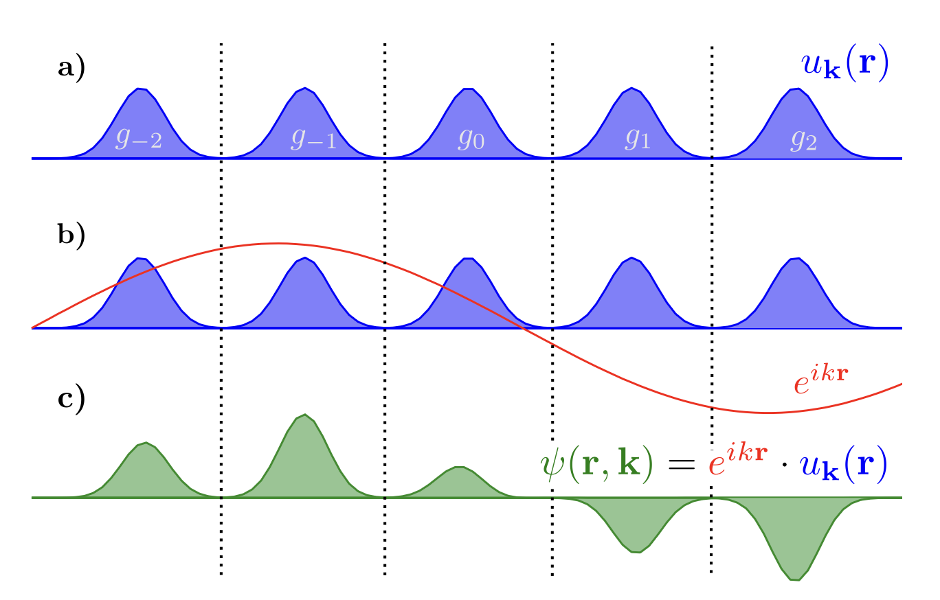
4. The Bloch Theorem#
Introduces the periodicity of the crystalline potential (of the unit cell) into the wave function:
\(k\) is the wave vector, \(\vec{k} = k_1\vec{b_1}+k_2\vec{b_2}+k_3\vec{b_3}\)
5. Plane-wave basis set#
For charge density:
Plane-wave:
[!NOTE]
PW vs LCAO:
PW:
+: Orthonormal
+: Independent of atomic positions
+: No basis set superposition errors (BSSE)
-: Large basis set (expensive to compute)
-: Hard to deal with localized orbitals
LCAO:
+: Chemistry insight
+: Small basis set (cheaper to compute)
-: not orthogonal
-: depends on atomic positions
-: BSSE
Plane-waves Cut-Off
Due to the PW expansion remains exact in the limit of an infinite number of G-vectors and all the plane waves fulfill the condition of orthonormality. However, in real situations, we can only have limit plane waves. To determine that:
6. DFT for Solids in the Plane-Wave Formalism#
In solids:
Choose \(E_\text{cutoff}\quad \&\quad\text{k-points grid}\)
Compute \(\rho(r)=\frac{1}{\Omega_{Bz}}\sum_n \int_{BZ}f_{nk}|\Psi_{nk}(r)|^2dk\)
7. Pseudopotential#
To deal with the external potential term \(V_\text{ne}\) : Plane wave is expensive since we need large basis set, the reason is \(V_\text{ne}(\vec{r_\text{ne}}) =-\frac{\mathcal{Z}_A}{|\vec{r_A}-\vec{r_i}|}\), when \(\vec{r_{ne}}\rightarrow 0\Rightarrow \text{singularity of } V_{ne}\), so, \(V_{ne}\) is very oscillate near core! It’s very hard to fit and needs more PW.
Examples:
Non-conserving PP (NCPP): integrated charge \(r<r_c\), same as all electron case
Ultrasoft PP (USPP): Relax norm-conservation then add augmentation charge to recover the correct charge density \(\rho\)
Projector augmented wave PP (PAW-PP): Reconstruct all electron wave function from pseudopotential using projectors.