Reinforcement Learning#
1. Proximal Policy Optimization (PPO)#
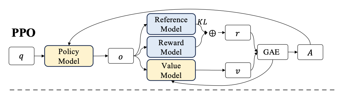
Proximal Policy Optimization (PPO) is an actor-critic RL algorithm that is widely used in the RL fine-tuning stage of LLMs. In particular, it optimizes LLMs by maximizing the following surrogate objective:
\(\theta\) is the parameter (weights) of the current policy model
\(\pi_\theta\) and \(\pi_{\theta_\text{old}}\) are the current and old policy models, also refers to the prob of generating token \(o_t\) given the context \(q\), under the current/old policy.
\(r_\theta=\frac{\pi_\theta(o_t|q)}{\pi_{\theta_\text{old}}(o_t|q)}\) is the probability ratio of the action under the current policy versus the old policy.
\(A_t\) is the advantage estimate at time \(t\), which is gained by GAE
\(\varepsilon\) is a small hyperparameter (e.g., 0.2) defining the clipping range. It prevents the rt(θ) ratio from moving too far from 1.0, ensuring safe, stable updates.
\(\text{clip}(x,\min,\max)\), if \(x<\min\), it output \(\min\); if \(x>\max\), it output \(\max\); Otherwise \(x\).
1.1. Generalized Advantage Estimation (GAE)#
To calculate the advantage, we apply Generalized Advantage Estimation (GAE) on the rewards \(r_t\) and a learned value function \(V_\omega\) given by critic (value) model.
Because we have this per-token reward \(r_t\), the Temporal Difference (TD) error calculation for the Critic at every step \(t\) :
[!TIP]
Tricks: Since it’s impossible to track the convergence of \(A_t=\sum_{l=0}^{T-t-1}(r\lambda)^l\delta_{t+l}\) to long sequence generation, e.g. \(t=1000\)
So, we set \(A_{t+1}=\sum_{l=0}^{T-t-2}(r\lambda)^l\sigma_{t+1+l}\)
So, \(A_t=\delta_t+ r\lambda A_{t+1}\)
\(\delta_t\): The TD error at step \(t\), calculated after the full trajectory is generated.
\(r_t\) is the step by step reward at \(t\) step
\(\gamma\) is the discount factor (usually around 0.99)
\(\lambda\): The GAE smoothing parameter (between 0 and 1). This is the magic dial that controls the bias-variance tradeoff.
\(l\): A counter index representing how many steps into the future we are looking.
The main idea of GAE is that, just like human intuition, like a long text page, the token at end of the page should has little correlation with the token in the middle, and it’s represented by \(\color{red}(r\lambda)^n\) which will decay at long sequence in GAE
1.2. Reward#
And the \(r_t\) is calculated by the reward function penalize the reward with KL compared with reference model at per-token level, since we don’t want to our model deviate too much from the pre-trained model in order to avoid the model crash for getting higher reward:
\(r_\phi\) is the reward model
\(\pi_\text{ref}\) is the reference model, which is usually the initial supervised fine-tuning (SFT) model
\(\beta\) is the coefficient of the KL penalty
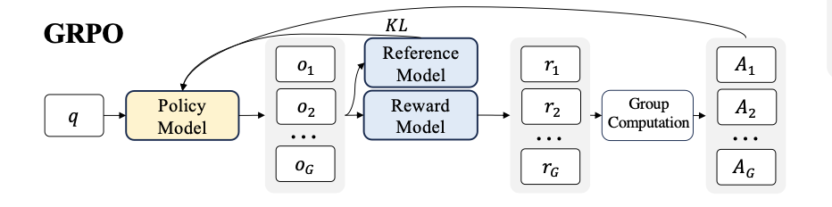
2. Group Relative Policy Optimization (GRPO)#
Since the value function is employed in PPO to mitigate over-optimization of the reward model, that model should has comparable size as policy model, which brings a substantial memory and computation burden. Additionally, during RL training, the value function is treated as a baseline in the calculation of the advantage for variance reduction.While in the LLM context, usually only the last token is assigned a reward score by the reward model, which may complicate the training of a value function that is accurate at each token.
Group Relative Policy Optimization (GRPO), which obviates the need for additional value function approximation as in PPO, and instead uses the average reward of multiple sampled outputs,
\(\alpha,\beta\) are hyper-parameters.
\(\hat{A}_{ij}\) is the advantage calculated based on relative rewards of the outputs inside each group only.
Also, to avoid the complicate calculation of advantage \(\hat{A}_{i,t}\), GRPO regularizes by directly adding the KL divergence between the trained policy and the reference policy to the loss.
Different from the KL penalty applied in PPO like equation (3), we estimate the KL divergence with the following unbiased estimator:
[!NOTE]
In LLM training practical, an LLM might has \(n+\) tokens, calculating the exact probabilities, doing softmax, summation, dividing, logging cost too much memory, so, instead calculating the norm probability, we estimate it using only the specific token \(\large o_{i,t}\) that the model actually chose to generate.
So, the naive estimator becomes: \(\log{\dfrac{\pi_\theta(o_{i,t}|q,o_{i<t})}{\pi_\text{ref}(o_{i,t}|q,o_{i,<t})}}\)
While the average (Expected Value) of this naive estimator will eventually equal the true KL divergence, a single calculation for a specific token can be negative. And if estimator output produces an negative value, we will subtract it and get a positive value, which will destroy the reward functions, leading to over-rewarding. Schulman proposed the formula in your image to fix this exact bug, as shown in equation 5: Let \(k=\dfrac{\pi_\text{ref}}{\pi_\theta}\), and the estimator will output: \(\text{Estimator}=k-\log{k}-1\), it’s Non-negative and produce some expectation value as the original KL divergence.
2.1. Process Supervision RL with GRPO#
Suppose for each question \(q\), we got a group of outputs \(\{o_1,...,o_G\}\) which are sampled from the old policy model \(\pi_\text{ref}\). A reward model will score the outputs and give reward scores \(\{r_1,...,r_G\}\). Subsequently, these rewards are normalized by subtracting the group average and dividing by the group standard deviation. Such outcome normalized reward at the end of each output \(\large o_i\) will be used for the advantage \(\hat{A_{i,t}}=\dfrac{r_i-r_\text{mean}}{\text{std(r)}}\). Then the final advantage will be \(A =\sum_l \hat{A_{i,t}^l}\), \(l\in K\) where \(l\) is the end token index and \(K\) is the total number of steps in the \(i\)-th output.
[1]: Shao, Z., Wang, P., Zhu, Q., Xu, R., Song, J., Bi, X., Zhang, H., Zhang, M., Li, Y.K., Wu, Y., Guo, D., 2024. DeepSeekMath: Pushing the Limits of Mathematical Reasoning in Open Language Models. https://doi.org/10.48550/arXiv.2402.03300