DFT2
1. Quick recap of DFT
Correlation energy: \(E^C = E^\text{exact}-E^\text{HF}\)
Electron density: \(\rho(r)\)
Functional: \(F[\rho(r)]\), input: function, output: value
Hohenberg-Kohn Theorem:
Kohn-Sham auxiliary system:
\(\hat{H}_\text{aux}=\hat{F}_\text{KS}=-\frac{1}{2}\nabla^2+V_\text{eff}(\vec{r})\)
2. The Kohn-Sham Variational Equations
Slater determinant:
\(H(\vec{x_1},...,\vec{x_N})=\frac{1}{\sqrt{N}}\begin{vmatrix}\theta_1(\vec{x_1}) & ...& \theta_N(\vec{x_1})\\\theta_N(\vec{x_N}) & ...& \theta_N(\vec{x_N})\end{vmatrix}\)
\[\begin{split}
\begin{align*}
&E_\text{KS}[\rho] = \underset{\text{non interacting kinetic}}{T_s[\rho]} + \underset{\text{external potential}}{\int d\vec{F}V_{ne}(\vec{r})\rho(\vec{r})}+ \underset{\text{Classical couomb interaction}}{E_\text{Hartree}[\rho]} + \underset{\text{exchange-correlation}}{E_xc[\rho]}\\
&= -\frac{1}{2} \sum_i^N \int d\mathbf{r}_1\, |\nabla \theta_i(\mathbf{r}_1, \sigma)|^2 - \sum_i^N \int \sum_A^M \frac{Z_A}{|\mathbf{r}_1 - \mathbf{R}_A|} |\theta_i(\mathbf{r}_1)|^2\\
&\quad + \frac{1}{2} \sum_i^N \sum_j^N \int \! \int d\mathbf{r}_1 d\mathbf{r}_2\,
|\theta_i(\mathbf{r}_1)|^2 \frac{1}{|\mathbf{r}_1 - \mathbf{r}_2|}
|\theta_j(\mathbf{r}_2)|^2
+ \underset{\text{unknown}}{E_{\mathrm{xc}}[\rho]}
\end{align*}
\end{split}\]
Again, the unknown term is \(E_{\mathrm{xc}}[\rho]\). Similarly as what we done in previous Hartree-Fock approximation session, we applied variational principle to make the orbitals \(\theta_i(r)\) fulfill in order to minimize this energy.
Recall that, variational principle \(\theta_i(r)\rightarrow \delta \theta_i(r), \delta \text{ is the variation factor}\)
\[\begin{split}
\hat{F}^\text{KS}\theta_i(r_1)=\epsilon \theta_i (r_1)\\
-\frac{1}{2}\nabla_1^2 + V_\text{eff}(r_1)
\end{split}\]
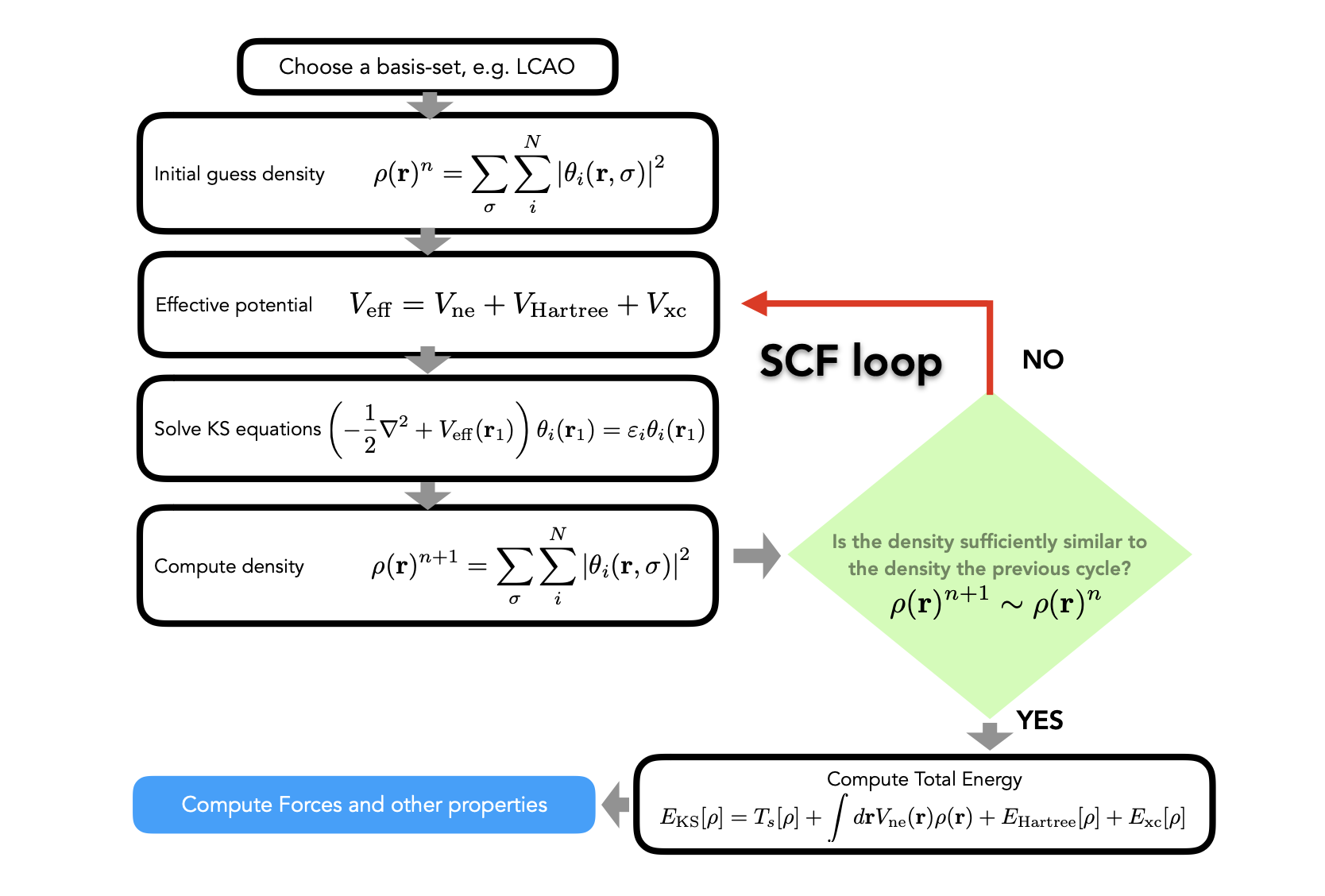
3. Achieving Self-Consistency of the Kohn-Sham Equations
\[
V_\text{eff} = \underset{\text{constant}}{V_\text{ne}}+\frac{\delta E_H[\rho]}{\delta \rho} +\frac{\delta E_\text{xc}[\rho]}{\delta \rho}
\]
4. Finding the Unknown Exchange-Correlation Functionals
\[\begin{split}
\left\{
\begin{aligned}
&\text{1. Chemist (empirical): get }E_\text{xc}\text{ by comparing to experiments}\\
&\text{e.g. heat of formation} \\
&\rightarrow\text{ energy does not guarantee a better functional or }\rho \\
&\text{2. Physicist: build from scratch (based on feature/constraints)}\\
&\rightarrow\text{ limited known features/constraints}
\end{aligned}
\right.
\end{split}\]
Local Density Approximation (LDA)
Assumption: uniform electron gas (metallic)
\[
E_\text{xc}^\text{LDA}=\int\rho(r)\epsilon_\text{xc}[\rho(r)]dr
\]
The quantity \(\epsilon_\text{xc}[\rho(r)]\) exchange and correlation contributions can be spilt as :
\[\begin{split}
\epsilon_\text{xc}[\rho(r)] = \underset{\text{exchange}}{\epsilon_\text{x}[\rho(r)]}+ \underset{\text{correlation}}{\epsilon_\text{c}[\rho(r)]}\\
\rightarrow \text{exchange: }\epsilon_x[\rho(r)]=-\frac{3}{4}\sqrt[3]{\frac{3\rho(r)}{\pi}}\\
\rightarrow \text{correlation: no explicit expression:}\\
\text{fit Quantum Monte Carlo}
\end{split}\]
Generalized Gradient Approximation (GGA)
\[
E_\text{xc}^\text{GGA}=\int f(\rho, \nabla\rho)dr
\]
The gradient itself It’s more like adding a Tylor expansion, the LDA method is the zero order of the series, while the gradient behaves as polynomials, making it more close the to value.
Meta-GGA
Rung-3 functional on Jacob’s ladder of DFT. It improves over GGA by using additional semilocal information about the electron density:
\[
E_\text{xc}^\text{meta-GGA} = \int f(\rho,\nabla \rho, \nabla^2 \rho,\tau)
\]
Kinetic energy density physical meanings:
It is large where orbitals oscillate rapidly (e.g. core, bonding), small where density is smooth.
bonding type (metallic, ionic, covalent)
iso-orbital regions (single-orbital like H atom)
weak interactions (vdW regions)